Multi-Resolution Function For Random Vibration Control
Product Overview
An Innovative Approach to Improve the Control Accuracy in the Low Frequency Range
Many characteristics of mechanical systems are better described logarithmically in the frequency domain. In vibration control tests, uniform frequency resolution that FFT offers is not ideal because the resolution is enough in the high-frequency range may be not enough in the low frequency and the control performance is impacted.
For example, many popular Random test standards require a profile up to 2 kHz and high resolution in the low-frequency range. To meet the requirement, high resolution (large block size) that is not needed in high frequency must be used. Therefore, loop time and storage space increase and spectrum refresh rate decrease in the high-frequency range.
To increase the control performance in the low-frequency range and maintain reasonable loop time, different resolutions should be applied to the low and high-frequency range in the entire control process.
EDM provides the multi-resolution feature that applies the selected resolution in the high-frequency range and 8 times of the resolution in the low-frequency range. The cutoff frequency, which divides the low and high-frequency range, is calculated by the software. A few adjacent frequencies can also be selected by the user to avoid system resonance or anti-resonance.
Product Resources
Control Algorithms
In the implementation, two different control loops with different sampling rates are used. Suppose that the sampling rate in the control system is Fs, we divide the whole frequency range into two bands: (0, Fs/20] and (Fs/20, Fh). DeltaF is the resolution in frequency band (Fs/20, Fh), then we use DeltaF/8 as the resolution in (0,Fs/20]. Down sampling 8 is used in the algorithm. Fig.2 shows us the multi-resolution control method to be used.
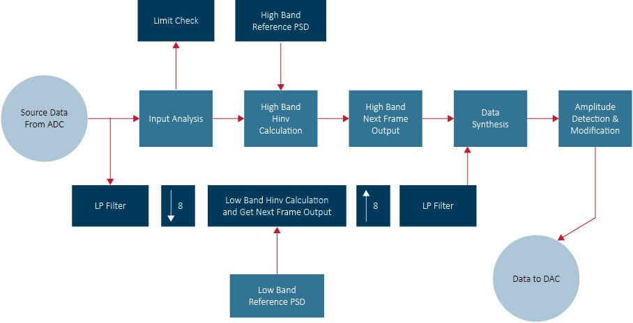
Figure 2: Two bands Multi-resolution Random Control
The output peak detection and modification also remain unchanged. In the CalOutput( ) function, we just add data from different bands, and send the result to the following detection and modification model, just as what in the now using system.
The user defined profile shall be decomposed into 2 bands in the initializing period, to get the low band reference profile. The Spider will operate on these two profiles simultaneously.
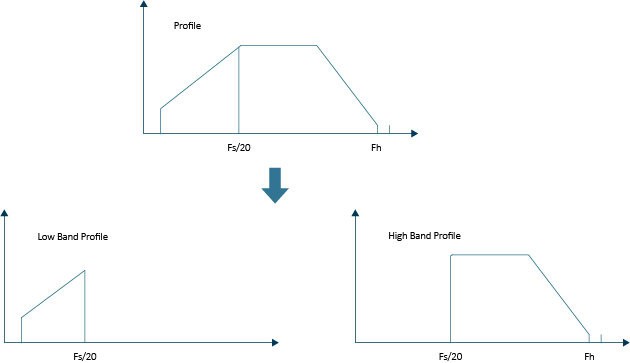
Figure 3: Profile divide into two bands
Testing Comparison
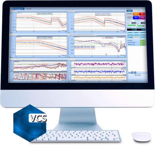
In the composite window below, a test is running without multi-resolution control at 400 lines.
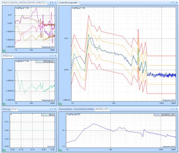
The blue line is the control spectrum. The green line is the profile spectrum. Yellow and red lines are alarm and abort limits.
In this case, a Spider is running a Random test with a profile where there are a few peaks and valleys below 100 Hz and between 200 to 500Hz. We can see that control spectrum matches the profile very well between 200 to 500Hz, but not satisfactory below 100Hz. The reason is described in the first paragraph of this article.
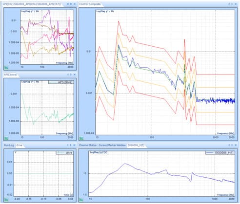
With multi-resolution control enabled, the resolution in the low-frequency range is much higher and the control performance is greatly improved. The control spectrum matches the profile below 100Hz as well as 200 to 500Hz.
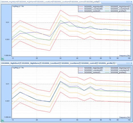
By zooming to 13~100Hz range in the control composite window in both cases.
The top chart shows how control(f) matches profile(f) WITHOUT multi-resolution control.
The bottom chart shows how control(f) matches profile(f) WITH multi-resolution control.
Control(f) matches profile(f) better with the multi-resolution control.
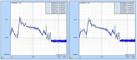
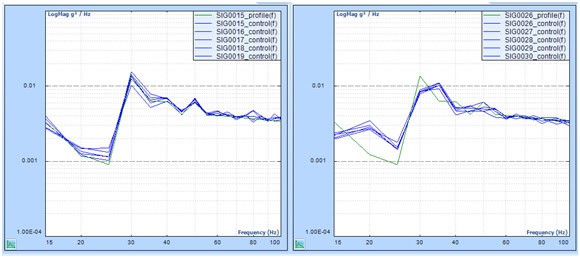
Here are more test results for comparison: (line = 400, Fa = 2000Hz, deltaF = 5Hz)
Signals in the left chart are saved in a Random test WITH multi-resolution.
Signals in the right chart are saved in a Random test WITHOUT multi-resolution.
Both charts show the frequency range of 10Hz to 2000Hz.
Zoom to 15 to 100Hz range
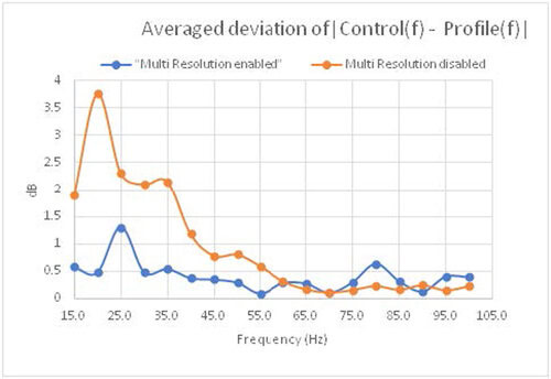
The following table shows the deviation in decibels between the control(f) and profile(f) (
Control(f)-Profile(f)
) at each FFT bin frequency.
Signal Name: SIG0015 SIG0016 SIG0017 SIG0018 SIG0019 Freq (Hz) profile (f) (dB) Control (f)-Profile(f)
(dB)
Average Control (f)-Profile (f)
(dB)
15.0 -24.75 0.82 0.70 0.13 0.43 0.82 0.58 20.0 -29.10 0.77 0.91 0.41 0.10 0.21 0.48 25.0 -30.46 2.21 1.64 1.02 1.08 0.57 1.31 30.0 -18.63 1.25 0.15 0.07 0.41 0.57 0.49 35.0 -22.02 0.82 0.51 0.21 0.19 0.99 0.54 40.0 -22.05 0.05 0.49 0.47 0.52 0.36 0.38 45.0 -23.77 0.58 0.37 0.06 0.30 0.45 0.35 50.0 -22.14 0.10 0.32 0.55 0.46 0.06 0.30 55.0 -23.77 0.14 0.05 0.02 0.09 0.21 0.10 60.0 -23.90 0.62 0.51 0.25 0.02 0.04 0.29 65.0 -24.02 0.09 0.21 0.25 0.59 0.26 0.28 70.0 -24.14 0.15 0.35 0.07 0.00 0.01 0.12 75.0 -24.24 0.39 0.35 0.36 0.22 0.22 0.31 80.0 -24.34 0.46 0.19 1.11 1.08 0.34 0.64 85.0 -24.43 0.38 0.54 0.49 0.11 0.10 0.32 90.0 -24.52 0.14 0.16 0.16 0.11 0.13 0.14 95.0 -24.60 0.06 0.31 0.27 0.94 0.46 0.41 100.0 -24.68 0.26 0.56 0.51 0.29 0.37 0.40 Signal Name: SIG0026 SIG0027 SIG0028 SIG0029 SIG0030 Freq (Hz) profile (f) (dB) Control (f)-Profile (f)
(dB)
Average Control (f)-Profile (f)
(dB)
15.0 -24.75 1.72 2.30 2.15 1.82 1.51 1.90 20.0 -29.10 3.44 3.33 3.68 4.50 3.89 3.77 25.0 -30.46 2.98 2.14 2.13 2.32 1.97 2.31 30.0 -18.63 1.86 2.03 2.14 2.39 2.10 2.10 35.0 -22.02 2.47 1.67 2.12 2.13 2.38 2.16 40.0 -22.05 0.79 1.79 0.93 1.24 1.16 1.18 45.0 -23.77 0.81 0.50 1.14 0.39 1.09 0.78 50.0 -22.14 0.91 1.22 1.24 0.63 0.04 0.81 55.0 -23.77 0.66 0.77 0.37 0.79 0.38 0.59 60.0 -23.90 0.53 0.14 0.37 0.21 0.37 0.32 65.0 -24.02 0.33 0.32 0.12 0.08 0.01 0.17 70.0 -24.14 0.08 0.02 0.24 0.06 0.17 0.12 75.0 -24.24 0.24 0.08 0.07 0.30 0.11 0.16 80.0 -24.34 0.13 0.65 0.31 0.02 0.05 0.23 85.0 -24.43 0.27 0.15 0.05 0.09 0.26 0.17 90.0 -24.52 0.32 0.04 0.21 0.12 0.54 0.25 95.0 -24.60 0.06 0.30 0.14 0.01 0.27 0.16 100.0 -24.68 0.21 0.12 0.05 0.15 0.63 0.23 Plot averaged difference of 5 signals at each frequency in both cases.
AutoShock-II: Automated Shock Test System
The AutoShock-II ™ is a fully automated series of shock...View Details
SD-Series: Mechanical Shock Machines
L.A.B. Equipment’s SD-Series mechanical shock machines provide precision testing for...View Details
Test Lab Professional™ Vibration v6 – USB
Test Lab Professional™ (TLP) is specifically designed to support the...View Details
Random Vibration Testing
The Random Vibration Control System provides precise, real-time, multi-channel control...View Details
Mix Mode Vibration Testing – SOR & ROR
Some vibration environments are characterized by quasi-periodic excitation from reciprocating...View Details
Swept Sine Vibration Testing
The Spider Swept Sine Vibration Control System provides precise, real-time,...View Details
Resonance Search and Dwell Test
The RSTD feature occurs in two phases. First, resonant frequencies...View Details
Multi-Sine Test
Multi-Sine Control allows for simultaneously sweeping multiple sine tones, helping...View Details
Shock Response Spectrum Synthesis & Control
The Shock Response Spectrum (SRS) vibration control package provides controls...View Details
Transient Time History Control
Generate or import transient time waveforms into EDM VCS for...View Details
Classic Shock Control
The Classic Shock vibration control feature provides precise, real-time, multi-channel...View Details
Transient Random Control
Transient Random Control drives a series of transient pulses to...View Details
Earthquake Testing Control
Vibration Tests for Seismic Qualification The earthquake testing control package...View Details

Multiple Shaker Control
EDM Multi-Shaker Control (MSC) is a software option included in...View Details
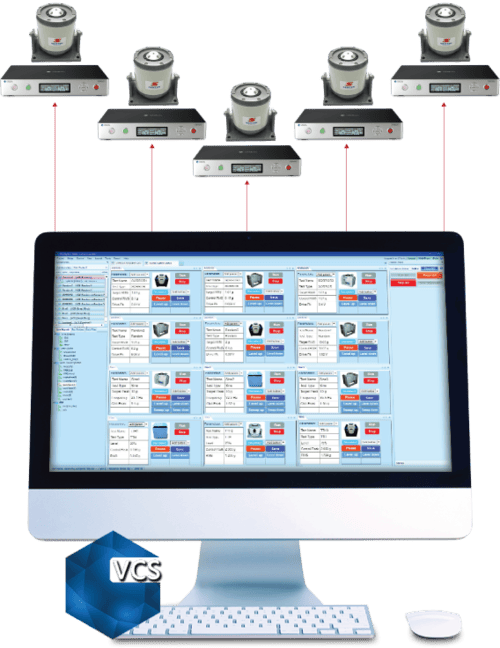
Vibration Visualization (VCS)
The 3D Model Reconstruction software produces 3D geometric models of...View Details
Multi-Resolution Function For Random Vibration Control
An Innovative Approach to Improve the Control Accuracy in the...View Details


MIMO Vibration Control
Multiple-Input Multiple-Output Vibration Control Software MIMO Testing has gained a...View DetailsFatigue Damage Spectrum
Fatigue Damage Spectrum (FDS) allows users to compare the potential...View DetailsMIMO Random Vibration Control
Multiple-Input Multiple-Output Random VCS The MIMO Random Control System provides...View Details
MIMO Sine Vibration Control
Multiple-Input Multiple-Output Sine VCS The MIMO Sine Control System provides...View Details
MIMO Classic Shock Vibration Control
Multiple-Input Multiple-Output Shock VCS The Spider MIMO Classic Shock Vibration...View Details
MIMO Transient Time History
Multiple-Input Multiple-Output TTH VCS Using template based importing tools, time...View DetailsMIMO Shock Response Spectrum
Multiple-Input Multiple-Output SRS VCS The Shock Response Spectrum vibration control...View Details
MIMO Time Waveform Replication
Multiple-Input Multiple-Output TWR Vibration Control MIMO Time Waveform Replication (TWR)...View Details

Precision Starts Here